


Normal Mapping
Advanced-Lighting/Normal-Mapping
All of our scenes are filled with meshes, each consisting of hundreds or maybe thousands of triangles. We boosted the realism by wrapping 2D textures on these flat triangles, hiding the fact that the polygons are just tiny flat triangles. Textures help, but when you take a good close look at the meshes it is still quite easy to see the underlying flat surfaces. Most real-life surface aren't flat however and exhibit a lot of (bumpy) details.
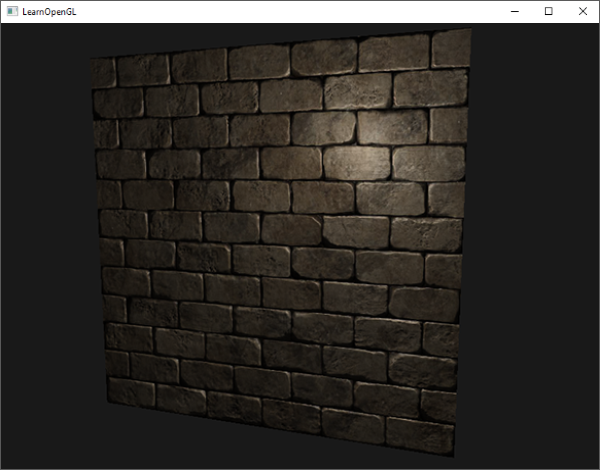
For instance, take a brick surface. A brick surface is quite a rough surface and obviously not completely flat: it contains sunken cement stripes and a lot of detailed little holes and cracks. If we were to view such a brick surface in a lit scene the immersion gets easily broken. Below we can see a brick texture applied to a flat surface lit by a point light.
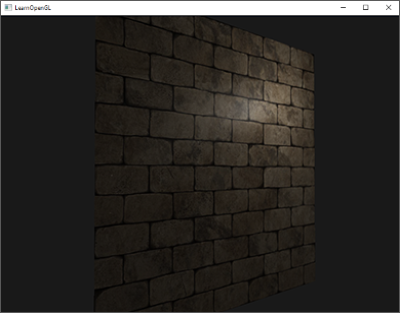
The lighting doesn't take any of the small cracks and holes into account and completely ignores the deep stripes between the bricks; the surface looks perfectly flat. We can partly fix the flat look by using a specular map to pretend some surfaces are less lit due to depth or other details, but that's more of a hack than a real solution. What we need is some way to inform the lighting system about all the little depth-like details of the surface.
If we think about this from a light's perspective: how comes the surface is lit as a completely flat surface? The answer is the surface's normal vector. From the lighting technique's point of view, the only way it determines the shape of an object is by its perpendicular normal vector. The brick surface only has a single normal vector, and as a result the surface is uniformly lit based on this normal vector's direction. What if we, instead of a per-surface normal that is the same for each fragment, use a per-fragment normal that is different for each fragment? This way we can slightly deviate the normal vector based on a surface's little details; this gives the illusion the surface is a lot more complex:

By using per-fragment normals we can trick the lighting into believing a surface consists of tiny little planes (perpendicular to the normal vectors) giving the surface an enormous boost in detail. This technique to use per-fragment normals compared to per-surface normals is called
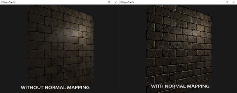
As you can see, it gives an enormous boost in detail and for a relatively low cost. Since we only change the normal vectors per fragment there is no need to change the lighting equation. We now pass a per-fragment normal, instead of an interpolated surface normal, to the lighting algorithm. The lighting then does the rest.
Normal mapping
To get normal mapping to work we're going to need a per-fragment normal. Similar to what we did with diffuse and specular maps we can use a 2D texture to store per-fragment normal data. This way we can sample a 2D texture to get a normal vector for that specific fragment.
While normal vectors are geometric entities and textures are generally only used for color information, storing normal vectors in a texture may not be immediately obvious. If you think about color vectors in a texture they are represented as a 3D vector with an r, g, and b component. We can similarly store a normal vector's x, y and z component in the respective color components. Normal vectors range between -1 and 1 so they're first mapped to [0,1]:
vec3 rgb_normal = normal * 0.5 + 0.5; // transforms from [-1,1] to [0,1]
With normal vectors transformed to an RGB color component like this, we can store a per-fragment normal derived from the shape of a surface onto a 2D texture. An example
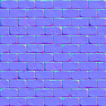
This (and almost all normal maps you find online) will have a blue-ish tint. This is because the normals are all closely pointing outwards towards the positive z-axis \((0, 0, 1)\): a blue-ish color. The deviations in color represent normal vectors that are slightly offset from the general positive z direction, giving a sense of depth to the texture. For example, you can see that at the top of each brick the color tends to be more greenish, which makes sense as the top side of a brick would have normals pointing more in the positive y direction \((0, 1, 0)\) which happens to be the color green!
With a simple plane, looking at the positive z-axis, we can take this diffuse texture and this normal map to render the image from the previous section. Note that the linked normal map is different from the one shown above. The reason for this is that OpenGL reads texture coordinates with the y (or v) coordinate reversed from how textures are generally created. The linked normal map thus has its y (or green) component inversed (you can see the green colors are now pointing downwards); if you fail to take this into account, the lighting will be incorrect. Load both textures, bind them to the proper texture units, and render a plane with the following changes in the lighting fragment shader:
uniform sampler2D normalMap;

void main()
{
    // obtain normal from normal map in range [0,1]
    normal = texture(normalMap, fs_in.TexCoords).rgb;
    // transform normal vector to range [-1,1]
    normal = normalize(normal * 2.0 - 1.0);

    [...]
    // proceed with lighting as normal
}
Here we reverse the process of mapping normals to RGB colors by remapping the sampled normal color from [0,1] back to [-1,1] and then use the sampled normal vectors for the upcoming lighting calculations. In this case we used a Blinn-Phong shader.
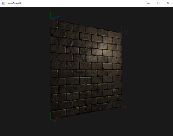
By slowly moving the light source over time you really get a sense of depth using the normal map. Running this normal mapping example gives the exact results as shown at the start of this chapter:
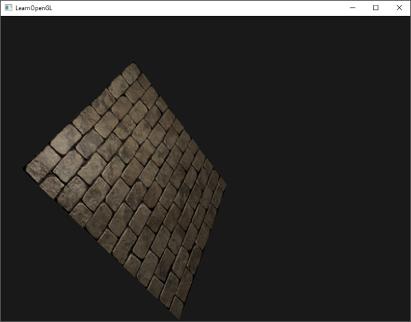
There is one issue however that greatly limits this use of normal maps. The normal map we used had normal vectors that all pointed somewhat in the positive z direction. This worked because the plane's surface normal was also pointing in the positive z direction. However, what would happen if we used the same normal map on a plane laying on the ground with a surface normal vector pointing in the positive y direction?
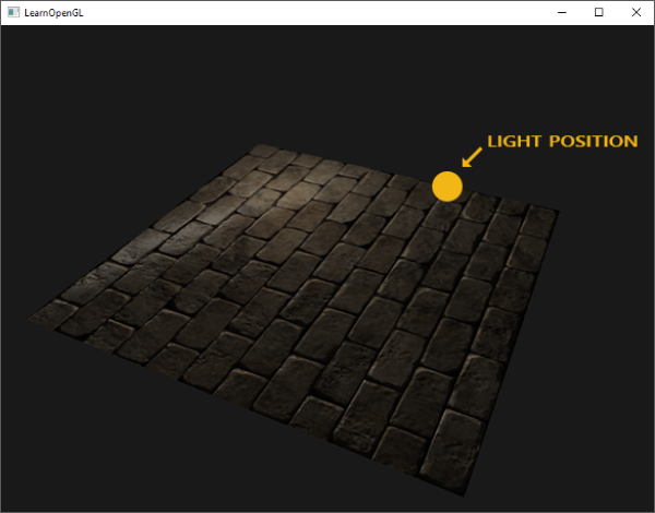
The lighting doesn't look right! This happens because the sampled normals of this plane still roughly point in the positive z direction even though they should mostly point in the positive y direction. As a result, the lighting thinks the surface's normals are the same as before when the plane was pointing towards the positive z direction; the lighting is incorrect. The image below shows what the sampled normals approximately look like on this surface:
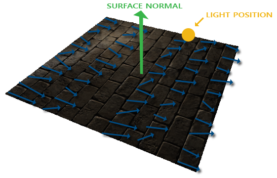
You can see that all the normals point somewhat in the positive z direction even though they should be pointing towards the positive y direction. One solution to this problem is to define a normal map for each possible direction of the surface; in the case of a cube we would need 6 normal maps. However, with advanced meshes that can have more than hundreds of possible surface directions this becomes an infeasible approach.
A different solution exists that does all the lighting in a different coordinate space: a coordinate space where the normal map vectors always point towards the positive z direction; all other lighting vectors are then transformed relative to this positive z direction. This way we can always use the same normal map, regardless of orientation. This coordinate space is called
Tangent space
Normal vectors in a normal map are expressed in tangent space where normals always point roughly in the positive z direction. Tangent space is a space that's local to the surface of a triangle: the normals are relative to the local reference frame of the individual triangles. Think of it as the local space of the normal map's vectors; they're all defined pointing in the positive z direction regardless of the final transformed direction. Using a specific matrix we can then transform normal vectors from this local tangent space to world or view coordinates, orienting them along the final mapped surface's direction.
Let's say we have the incorrect normal mapped surface from the previous section looking in the positive y direction. The normal map is defined in tangent space, so one way to solve the problem is to calculate a matrix to transform normals from tangent space to a different space such that they're aligned with the surface's normal direction: the normal vectors are then all pointing roughly in the positive y direction. The great thing about tangent space is that we can calculate this matrix for any type of surface so that we can properly align the tangent space's z direction to the surface's normal direction.
Such a matrix is called a
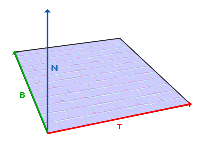
We already know the up vector, which is the surface's normal vector. The right and forward vector are the tangent and bitangent vector respectively. The following image of a surface shows all three vectors on a surface:
Calculating the tangent and bitangent vectors is not as straightforward as the normal vector. We can see from the image that the direction of the normal map's tangent and bitangent vector align with the direction in which we define a surface's texture coordinates. We'll use this fact to calculate tangent and bitangent vectors for each surface. Retrieving them does require a bit of math; take a look at the following image:
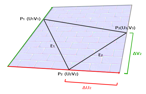
From the image we can see that the texture coordinate differences of an edge \(E_2\) of a triangle (denoted as \(\Delta U_2\) and \(\Delta V_2\)) are expressed in the same direction as the tangent vector \(T\) and bitangent vector \(B\). Because of this we can write both displayed edges \(E_1\) and \(E_2\) of the triangle as a linear combination of the tangent vector \(T\) and the bitangent vector \(B\):
\[E_1 = \Delta U_1T + \Delta V_1B\] \[E_2 = \Delta U_2T + \Delta V_2B\]Which we can also write as:
\[(E_{1x}, E_{1y}, E_{1z}) = \Delta U_1(T_x, T_y, T_z) + \Delta V_1(B_x, B_y, B_z)\] \[(E_{2x}, E_{2y}, E_{2z}) = \Delta U_2(T_x, T_y, T_z) + \Delta V_2(B_x, B_y, B_z)\]We can calculate \(E\) as the difference vector between two triangle positions, and \(\Delta U\) and \(\Delta V\) as their texture coordinate differences. We're then left with two unknowns (tangent \(T\) and bitangent \(B\)) and two equations. You may remember from your algebra classes that this allows us to solve for \(T\) and \(B\).
The last equation allows us to write it in a different form: that of matrix multiplication:
\[\begin{bmatrix} E_{1x} & E_{1y} & E_{1z} \\ E_{2x} & E_{2y} & E_{2z} \end{bmatrix} = \begin{bmatrix} \Delta U_1 & \Delta V_1 \\ \Delta U_2 & \Delta V_2 \end{bmatrix} \begin{bmatrix} T_x & T_y & T_z \\ B_x & B_y & B_z \end{bmatrix} \]Try to visualize the matrix multiplications in your head and confirm that this is indeed the same equation. An advantage of rewriting the equations in matrix form is that solving for \(T\) and \(B\) is easier to understand. If we multiply both sides of the equations by the inverse of the \(\Delta U \Delta V\) matrix we get:
\[ \begin{bmatrix} \Delta U_1 & \Delta V_1 \\ \Delta U_2 & \Delta V_2 \end{bmatrix}^{-1} \begin{bmatrix} E_{1x} & E_{1y} & E_{1z} \\ E_{2x} & E_{2y} & E_{2z} \end{bmatrix} = \begin{bmatrix} T_x & T_y & T_z \\ B_x & B_y & B_z \end{bmatrix} \]This allows us to solve for \(T\) and \(B\). This does require us to calculate the inverse of the delta texture coordinate matrix. I won't go into the mathematical details of calculating a matrix' inverse, but it roughly translates to 1 over the determinant of the matrix, multiplied by its adjugate matrix:
\[ \begin{bmatrix} T_x & T_y & T_z \\ B_x & B_y & B_z \end{bmatrix} = \frac{1}{\Delta U_1 \Delta V_2 - \Delta U_2 \Delta V_1} \begin{bmatrix} \Delta V_2 & -\Delta V_1 \\ -\Delta U_2 & \Delta U_1 \end{bmatrix} \begin{bmatrix} E_{1x} & E_{1y} & E_{1z} \\ E_{2x} & E_{2y} & E_{2z} \end{bmatrix} \]This final equation gives us a formula for calculating the tangent vector \(T\) and bitangent vector \(B\) from a triangle's two edges and its texture coordinates.
Don't worry if you do not fully understand the mathematics behind this. As long as you understand that we can calculate tangents and bitangents from a triangle's vertices and its texture coordinates (since texture coordinates are in the same space as tangent vectors) you're halfway there.
Manual calculation of tangents and bitangents
In the previous demo we had a simple normal mapped plane facing the positive z direction. This time we want to implement normal mapping using tangent space so we can orient this plane however we want and normal mapping would still work. Using the previously discussed mathematics we're going to manually calculate this surface's tangent and bitangent vectors.
Let's assume the plane is built up from the following vectors (with 1, 2, 3 and 1, 3, 4 as its two triangles):
// positions
glm::vec3 pos1(-1.0,  1.0, 0.0);
glm::vec3 pos2(-1.0, -1.0, 0.0);
glm::vec3 pos3( 1.0, -1.0, 0.0);
glm::vec3 pos4( 1.0,  1.0, 0.0);
// texture coordinates
glm::vec2 uv1(0.0, 1.0);
glm::vec2 uv2(0.0, 0.0);
glm::vec2 uv3(1.0, 0.0);
glm::vec2 uv4(1.0, 1.0);
// normal vector
glm::vec3 nm(0.0, 0.0, 1.0);
We first calculate the first triangle's edges and delta UV coordinates:
glm::vec3 edge1 = pos2 - pos1;
glm::vec3 edge2 = pos3 - pos1;
glm::vec2 deltaUV1 = uv2 - uv1;
glm::vec2 deltaUV2 = uv3 - uv1;
With the required data for calculating tangents and bitangents we can start following the equation from the previous section:
float f = 1.0f / (deltaUV1.x * deltaUV2.y - deltaUV2.x * deltaUV1.y);

tangent1.x = f * (deltaUV2.y * edge1.x - deltaUV1.y * edge2.x);
tangent1.y = f * (deltaUV2.y * edge1.y - deltaUV1.y * edge2.y);
tangent1.z = f * (deltaUV2.y * edge1.z - deltaUV1.y * edge2.z);

bitangent1.x = f * (-deltaUV2.x * edge1.x + deltaUV1.x * edge2.x);
bitangent1.y = f * (-deltaUV2.x * edge1.y + deltaUV1.x * edge2.y);
bitangent1.z = f * (-deltaUV2.x * edge1.z + deltaUV1.x * edge2.z);

[...] // similar procedure for calculating tangent/bitangent for plane's second triangle
Here we first pre-calculate the fractional part of the equation as f and then for each vector component we do the corresponding matrix multiplication multiplied by f. If you compare this code with the final equation you can see it is a direct translation. Because a triangle is always a flat shape, we only need to calculate a single tangent/bitangent pair per triangle as they will be the same for each of the triangle's vertices.
The resulting tangent and bitangent vector should have a value of (1,0,0) and (0,1,0) respectively that together with the normal (0,0,1) forms an orthogonal TBN matrix. Visualized on the plane, the TBN vectors would look like this:
With tangent and bitangent vectors defined per vertex we can start implementing proper normal mapping.
Tangent space normal mapping
To get normal mapping working, we first have to create a TBN matrix in the shaders. To do that, we pass the earlier calculated tangent and bitangent vectors to the vertex shader as vertex attributes:
#version 330 core
layout (location = 0) in vec3 aPos;
layout (location = 1) in vec3 aNormal;
layout (location = 2) in vec2 aTexCoords;
layout (location = 3) in vec3 aTangent;
layout (location = 4) in vec3 aBitangent;
Then within the vertex shader's
void main()
{
   [...]
   vec3 T = normalize(vec3(model * vec4(aTangent,   0.0)));
   vec3 B = normalize(vec3(model * vec4(aBitangent, 0.0)));
   vec3 N = normalize(vec3(model * vec4(aNormal,    0.0)));
   mat3 TBN = mat3(T, B, N);
}
Here we first transform all the TBN vectors to the coordinate system we'd like to work in, which in this case is world-space as we multiply them with the model matrix. Then we create the actual TBN matrix by directly supplying
vec3 B = cross(N, T);
So now that we have a TBN matrix, how are we going to use it? There are two ways we can use a TBN matrix for normal mapping, and we'll demonstrate both of them:
- We take the TBN matrix that transforms any vector from tangent to world space, give it to the fragment shader, and transform the sampled normal from tangent space to world space using the TBN matrix; the normal is then in the same space as the other lighting variables.
- We take the inverse of the TBN matrix that transforms any vector from world space to tangent space, and use this matrix to transform not the normal, but the other relevant lighting variables to tangent space; the normal is then again in the same space as the other lighting variables.
Let's review the first case. The normal vector we sample from the normal map is expressed in tangent space whereas the other lighting vectors (light and view direction) are expressed in world space. By passing the TBN matrix to the fragment shader we can multiply the sampled tangent space normal with this TBN matrix to transform the normal vector to the same reference space as the other lighting vectors. This way, all the lighting calculations (specifically the dot product) make sense.
Sending the TBN matrix to the fragment shader is easy:
out VS_OUT {
    vec3 FragPos;
    vec2 TexCoords;
    mat3 TBN;
} vs_out;

void main()
{
    [...]
    vs_out.TBN = mat3(T, B, N);
}
In the fragment shader we similarly take a mat3 as an input variable:
in VS_OUT {
    vec3 FragPos;
    vec2 TexCoords;
    mat3 TBN;
} fs_in;
With this TBN matrix we can now update the normal mapping code to include the tangent-to-world space transformation:
normal = texture(normalMap, fs_in.TexCoords).rgb;
normal = normal * 2.0 - 1.0;
normal = normalize(fs_in.TBN * normal);
Because the resulting normal is now in world space, there is no need to change any of the other fragment shader code as the lighting code assumes the normal vector to be in world space.
Let's also review the second case, where we take the inverse of the TBN matrix to transform all relevant world-space vectors to the space the sampled normal vectors are in: tangent space. The construction of the TBN matrix remains the same, but we first invert the matrix before sending it to the fragment shader:
vs_out.TBN = transpose(mat3(T, B, N));
Note that we use the
Within the fragment shader we do not transform the normal vector, but we transform the other relevant vectors to tangent space, namely the lightDir and viewDir vectors. That way, each vector is in the same coordinate space: tangent space.
void main()
{
    vec3 normal = texture(normalMap, fs_in.TexCoords).rgb;
    normal = normalize(normal * 2.0 - 1.0);

    vec3 lightDir = fs_in.TBN * normalize(lightPos - fs_in.FragPos);
    vec3 viewDir  = fs_in.TBN * normalize(viewPos - fs_in.FragPos);
    [...]
}
The second approach looks like more work and also requires matrix multiplications in the fragment shader, so why would we bother with the second approach?
Well, transforming vectors from world to tangent space has an added advantage in that we can transform all the relevant lighting vectors to tangent space in the vertex shader instead of in the fragment shader. This works, because lightPos and viewPos don't update every fragment run, and for fs_in.FragPos we can calculate its tangent-space position in the vertex shader and let fragment interpolation do its work. There is effectively no need to transform a vector to tangent space in the fragment shader, while it is necessary with the first approach as sampled normal vectors are specific to each fragment shader run.
So instead of sending the inverse of the TBN matrix to the fragment shader, we send a tangent-space light position, view position, and vertex position to the fragment shader. This saves us from having to do matrix multiplications in the fragment shader. This is a nice optimization as the vertex shader runs considerably less often than the fragment shader. This is also the reason why this approach is often the preferred approach.
out VS_OUT {
    vec3 FragPos;
    vec2 TexCoords;
    vec3 TangentLightPos;
    vec3 TangentViewPos;
    vec3 TangentFragPos;
} vs_out;

uniform vec3 lightPos;
uniform vec3 viewPos;

[...]

void main()
{
    [...]
    mat3 TBN = transpose(mat3(T, B, N));
    vs_out.TangentLightPos = TBN * lightPos;
    vs_out.TangentViewPos  = TBN * viewPos;
    vs_out.TangentFragPos  = TBN * vec3(model * vec4(aPos, 1.0));
}
In the fragment shader we then use these new input variables to calculate lighting in tangent space. As the normal vector is already in tangent space, the lighting makes sense.
With normal mapping applied in tangent space, we should get similar results to what we had at the start of this chapter. This time however, we can orient our plane in any way we'd like and the lighting would still be correct:
glm::mat4 model = glm::mat4(1.0f);
model = glm::rotate (model, (float)glfwGetTime () * -10.0f, glm::normalize(glm::vec3(1.0, 0.0, 1.0)));
shader.setMat4("model", model);
RenderQuad();
Which indeed looks like proper normal mapping:
You can find the source code here.
Complex objects
We've demonstrated how we can use normal mapping, together with tangent space transformations, by manually calculating the tangent and bitangent vectors. Luckily for us, having to manually calculate these tangent and bitangent vectors is not something we do too often. Most of the time you implement it once in a custom model loader, or in our case use a model loader using Assimp.
Assimp has a very useful configuration bit we can set when loading a model called aiProcess_CalcTangentSpace. When the aiProcess_CalcTangentSpace bit is supplied to Assimp's
const aiScene *scene = importer.ReadFile(
    path, aiProcess_Triangulate | aiProcess_FlipUVs | aiProcess_CalcTangentSpace
);
Within Assimp we can then retrieve the calculated tangents via:
vector.x = mesh->mTangents[i].x;
vector.y = mesh->mTangents[i].y;
vector.z = mesh->mTangents[i].z;
vertex.Tangent = vector;
Then you'll have to update the model loader to also load normal maps from a textured model. The wavefront object format (.obj) exports normal maps slightly different from Assimp's conventions as aiTextureType_NORMAL doesn't load normal maps, while aiTextureType_HEIGHT does:
vector<Texture> normalMaps = loadMaterialTextures(material, aiTextureType_HEIGHT, "texture_normal");
Of course, this is different for each type of loaded model and file format.
Running the application on a model with specular and normal maps, using an updated model loader, gives the following result:
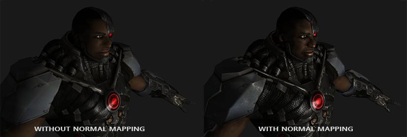
As you can see, normal mapping boosts the detail of an object by an incredible amount without too much extra cost.
Using normal maps is also a great way to boost performance. Before normal mapping, you had to use a large number of vertices to get a high number of detail on a mesh. With normal mapping, we can get the same level of detail on a mesh using a lot less vertices. The image below from Paolo Cignoni shows a nice comparison of both methods:
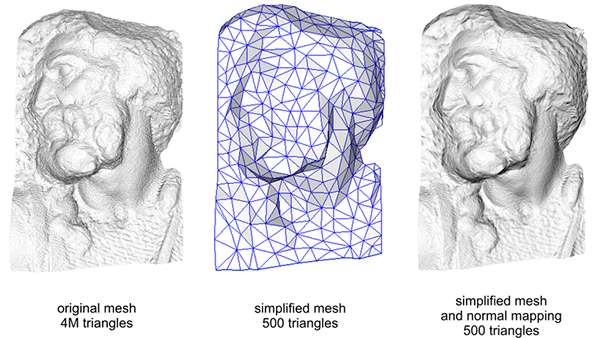
The details on both the high-vertex mesh and the low-vertex mesh with normal mapping are almost indistinguishable. So normal mapping doesn't only look nice, it's a great tool to replace high-vertex meshes with low-vertex meshes without losing (too much) detail.
One last thing
There is one last trick left to discuss that slightly improves quality without too much extra cost.
When tangent vectors are calculated on larger meshes that share a considerable amount of vertices, the tangent vectors are generally averaged to give nice and smooth results. A problem with this approach is that the three TBN vectors could end up non-perpendicular, which means the resulting TBN matrix would no longer be orthogonal. Normal mapping would only be slightly off with a non-orthogonal TBN matrix, but it's still something we can improve.
Using a mathematical trick called the
vec3 T = normalize(vec3(model * vec4(aTangent, 0.0)));
vec3 N = normalize(vec3(model * vec4(aNormal, 0.0)));
// re-orthogonalize T with respect to N
T = normalize(T - dot(T, N) * N);
// then retrieve perpendicular vector B with the cross product of T and N
vec3 B = cross(N, T);

mat3 TBN = mat3(T, B, N)
This, albeit by a little, generally improves the normal mapping results with a little extra cost. Take a look at the end of the Normal Mapping Mathematics video in the additional resources for a great explanation of how this process actually works.
Additional resources
- Tutorial 26: Normal Mapping: normal mapping tutorial by ogldev.
- How Normal Mapping Works: a nice video tutorial of how normal mapping works by TheBennyBox.
- Normal Mapping Mathematics: a similar video by TheBennyBox about the mathematics behind normal mapping.
- Tutorial 13: Normal Mapping: normal mapping tutorial by opengl-tutorial.org.