Area Lights

Sponza scene illuminated by a textured, rectangular area light. [1]

Introduction

We want lights. And we want them everywhere. In the basic tutorial series 3 distinct light types have been presented thoroughly: directional lights, point lights, and spotlights. And while we can achieve good results with them, they all have a major drawback: Light sources in the real world are (almost) never restricted to a single (infinitely-small) point - rather they usually cover an area.

But we cannot easily represent such a light source using those 3 basic types of light. Imagine if we wanted to display a rectangular light source: It would require us to place hundreds, if not thousands, of tiny spot lights next to each other in a close uniform grid. Besides the obvious loss of rendering efficiency the result would likely not be very good, and if the camera would be very close to the area light source we would probably need even more small lights in that area. And this is not even taking into account the amount of over- illumination which would most likely appear, so each light would have to be dimmed quite a lot for all these lights to give a combined, realistic appearance. Clearly, this is not desirable.
With raytracing this problem can be solved quite straight-forward by Monte-Carlo sampling, but assuming most readers in here are interested in real-time applications (ie. games), this is not really of much relevance to us. (yet!)

This tutorial describes how to render area light sources from arbitrarily convex polygons using a method called ”Linearly Transformed Cosines”, originally published in 2016 by Eric Heitz, Jonathan Dupuy, Stephen Hill, and David Neubelt. Later extensions have been made to this method to support circular shapes in addition to rectangular or sharp-edged polygons.

In this article, we will look at the theory behind implementing rectangular area lights.

Prerequisites

This method builds upon physically-based rendering techniques (PBR), so familiarity with the core concepts is recommended for an optimal learning experience. It is also very math-heavy, so familiarity with several mathematical concepts is recommended for a full learning experience, including: Integrals, linear algebra, trigonometry, solid angle measurement, and distributions. But if you simply want to implement it and see it working then you may copy/paste the code snippets. This stuff is very advanced, and while studying the mathematics can be worthwhile, you are certainly not expected to understand it all. Some clever researchers did the hard work for us, so that our rendering applications can look cool! :)
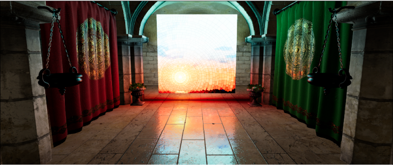
You may also have noticed that the cover image has a textured light source. This article will not go into details on how to accomplish this, although it might be touched upon in a future chapter. So let's get started...

Problem description

Let’s say we have a scene, and we place a rectangle in the scene at some position in close proximity to our game objects. We wish for this rectangle to represent a light source and thus, emit light. We also have our BRDF, which describes how the surfaces in the scene scatter light.
So given incoming radiance from the light source around a given shading point (ie. a fragment), we need to solve the integral of the BRDF, over the spherical polygon, as the solid angle of the light source polygon subtended at the unit hemisphere around the shading point, to calculate the outgoing radiance. This outgoing radiance is what will reflect back to our eyes and thusly illuminate the scene.
The article which introduced this method describes how a linear transformation, represented by a 3x3 matrix, can be applied to a distribution thus yielding a new family of distributions which share some core properties. These properties are very well-explained in Eric Heitz’ presentation slides [3]. But since this is meant to be a programming guide primarily, we will not discuss their derivations here. The new family of distributions have been conveniently dubbed ”Linearly Transformed Cosines”, because a clamped cosine distribution (by choice) has been applied a linear transformation, while retaining the important properties which makes them a suitable approximation to physically-based BRDFs. ”Clamped” refers to a cosine distribution (or ”Lambertian” distribution), which has been clamped to the hemisphere. This is important since unit sphere solid angle measures are in the interval [0, 4π], while a light source should probably never illuminate objects facing away from them; thus we clamp the distribution to the ”upper” hemisphere (oriented around the surface normal of the incident shading point).

Well-known BRDFs, such as the GGX microfacet model, have sophisticated shapes that support anisotropic stretching at grazing angles, skewness, and varying degrees of material roughnesses, among others. It is due to these properties that BRDFs yield realistically-looking results. So if we can design a linear transformation that adds these properties to the cosine distribution, through matrix-multiplication, then we can obtain these desired properties. The article [1] describes how this is possible. The cosine distribution is a very good choice because we have a closed-form representation of its integral:

\[ D_o(\omega_o) = \dfrac{1}{\pi}cos \theta_o \]

In summary, our strategy is this: Construct a 3x3 matrix which represents our BRDF, use it to transform a clamped cosine distribution, and then compute the solid angle measure through the closed-form representation.

You may remember from linear algebra that if we multiply two matrices A and B, we may also perform an ”inverse” operation (given that B is invertible):

\[ A \times B = C \qquad \Leftrightarrow \qquad C \times B^{-1} = A \]

If our linear transformation matrix, M, is applied to our cosine distribution to yield our BRDF-approximation, then we may compute in reverse order, allowing us to elegantly solve the integral. This idea is illustrated below. As the authors suggest, we may think of this as transforming back to cosine space.

Inverse transformation back to cosine space, using the inverse linear transformation matrix. Taken from [2].

Construction of the transformation matrix

The linear transformation matrix M needs to represent the BRDF, parameterized over both the viewing angle and the material roughness. The following images illustrate the idea:

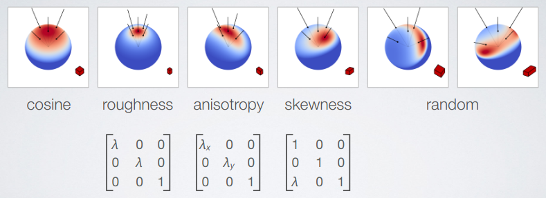
Constructing the linear transformation by a chained matrix-multiplication to represent desired features of a BRDF. [2]

The roughness parameter is directly translated to the value from the material’s roughness texture found in a typical PBR-pipeline, and the anisotropy and skewness stretches and skews the reflected highlight at increasingly grazing viewing angles for realistic renderings. As illustrated, we may choose an arbitrary amount of transformations, depending on our requirements and the specific BRDF model we wish to represent. In this tutorial we will use a matrix which approximates (but not perfectly replicates) the GGX microfacet model. As mentioned, we need 1 matrix M, for each combination of material roughness and viewing angle, which directly translates to 1 matrix M for each shaded fragment! Not only that, but we need to sample the matrix several times and minimize the error compared to our chosen BRDF. Clearly, this is not doable for real-time purposes, so the matrix M needs to be precomputed for each roughness/view-angle pair. Since both the matrix M and its inverse are sparse matrices with 5 non-zero values, we can store the inverted matrix in a 4-vector by normalizing by the middle field. This works well in pratice and neatly allows us to send the matrices to the GPU in a 2D-texture. We choose a 64x64 texture to save memory bandwith, and because it yields acceptable results.

Computing the integral

To compute the integral, we can calculate a sum of integrals over the boundary edges of the spherical polygon. This may sound like sorcery, and without making this tutorial too lengthy I will quote the presentation slides [2] and encourage the reader to investigate further:

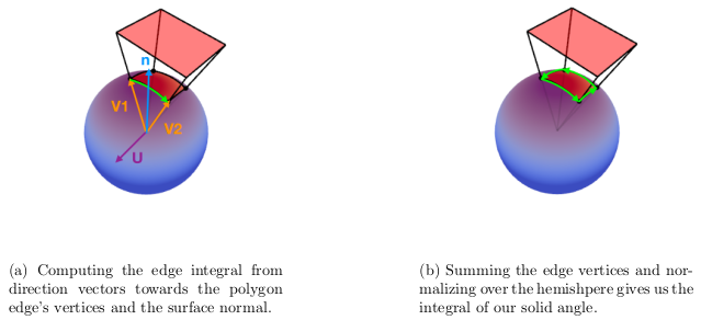
”One way to think about it is as an application of Stoke’s theorem, which you might have encountered in other areas, such as fluid simulation.”

Stoke's Theorem states that "a line integral of a vector field over a loop is equal to the flux of its curl through the enclosed surface." (source: Wikipedia [11]). Given a boundary edge of the polygon, defined by vertices v1 and v2, we calculate the edge’s integral as follows:

\[ acos(v_1 \cdot v_2) \dfrac{v_1 \times v_2}{|| v_1 \times v_2 ||} \cdot n \]

And for a light polygon with N edges we can quite accurately calculate the solid angle of the polygon by summing the edge integrals:

\[ \int_{\Omega}\, \approx \, \frac{1}{2\pi} \sum_{i=1}^{N} \left[ acos(v_1 \cdot v_2) \dfrac{v_1 \times v_2}{|| v_1 \times v_2 ||} \cdot n \right] \]

Here the vectors v1 and v2 are direction vectors from the shading point to the polygon edge’s vertices, the ”acos(v1 · v2 )” is the arc length in radians of the polygon edge projected onto the unit sphere situated about the shading point, and the normalized cross product yields a vector, u, which is perpendicular to v1 and v2 . We dot with the normal vector of the shading point to project onto the plane that is tangent to the shading point and which has normal vector n.

The subtended area integral is computed from the sum of edge integrals, by application of Stoke's Theorem. Images taken from [2].

As described in [2], the authors found significant visual artifacts when computing the edge integrals, because of missing precision found in the acos function. So instead they introduced a cubic function which approximates acos. The function for calculating the edge integral with the cubic function is shown below in glsl-code. This function differs from the cubic fit originally introduced in [2]. This optimized version is a later iteration, and yields a better fit.

vec3 IntegrateEdge(vec3 v1, vec3 v2, vec3 N) {
    float x = dot(v1, v2);
    float y = abs(x);
    float a = 0.8543985 + (0.4965155 + 0.0145206*y)*y;
    float b = 3.4175940 + (4.1616724 + y)*y;
    float v = a / b;
    float theta sintheta = (x > 0.0) ? v : 0.5*inversesqrt(max(1.0 - x*x, 1e-7)) - v;
    return dot(cross(v1, v2)*theta sintheta, N);
}

Clip polygon to upper hemisphere

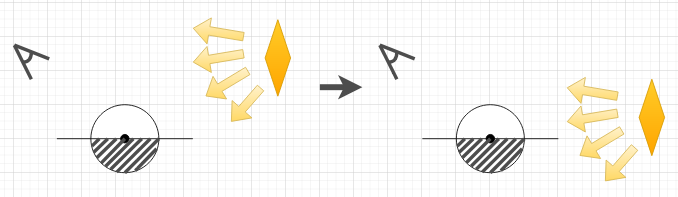
The IntegrateEdge function shown above is, although a very good solution, not perfect. In order to get the correct radiance calculation we need to clamp the transformed cosine distribution to the upper hemisphere. This process may also be referred to as ”horizon-clipping”, and involves a lot of branching. See this image below:

If the light source moves below, or partially below, the horizon, it needs to be clipped, which in practice involves moving the lower vertices of each edge upwards such that they are no longer below the horizon. And if an edge is entirely situated below the horizon its vertices will be situated atop of each other. In either case the computed edge integral will yield a lower (or possibly zero) value resulting in less outgoing radiance. But if we need to make a comparison for each vertex of all edges then we will end up with heavily branched code, which is always bad in a fragment shader. So instead we will modify our formula for the edge integral by removing the dot product with the surface normal (and thus not project onto the plane). The formula now looks like this:

\[ acos(v_1 \cdot v_2) \dfrac{v_1 \times v_2}{|| v_1 \times v_2 ||} \]

This gives us a vector form instead, which we may think of as a vector form factor, or vector irradiance, and it has a neat property: The length of this vector is the form factor of the light polygon, in the direction of this vector. Let’s call this vector ”F ”. We can use F to compute the angular extent and elevation angle by constructing a ”proxy sphere” around our current shading point. The formulas are shown below:

\[ F = acos(v_1 \cdot v_2) \dfrac{v_1 \times v_2}{|| v_1 \times v_2 ||} \] \[ length(F) \rightarrow \text{form factor in direction of } F \] \[ \text{angular extent} = asin(sqrt(length(F)) \] \[ \text{elevation angle} = dot(N, normalize(F)) \]

This can help us since we have a couple of analytical solutions for horizon-clipped sphere form factors. So by precomputing the form factors for spheres of different angular extents and elevation angles, we can make an additional texture lookup at runtime to fetch clipped form factors, thereby efficiently solving our problem of horizon-clipping by close approximation. More details are found in the slides [2], as well as in the article [1].

A form factor is an expression of the amount of outgoing energy or "radiance", which emitted from a patch A1 reaches another patch A2. This is quite similar to how we subtend the area light polygon on a half-sphere around each shading point. Each form factor is stored in a 64x64 LUT, indexed by angular extent and elevation angle. We are using the term irradiance, because we focus on the incoming light energi. A more comprehensive introduction to form factors may be found in [13].

Putting it all together

Congratulations if you were able to follow along so far. This is quite math heavy, so don’t worry if you didn’t understand everything. You may safely copy/paste the code examples and get it working yourself, and if you are feeling adventurous then you are warmly recommended to go through the source material yourself, linked at the bottom of this page. The mathematics will never lose relevance. But for now, let’s progress to the fun part! :) Our first step is loading the matrices onto the GPU as 2D-textures. We should remember to enable bilinear filtering for the smoothest results, and edge-clamping in case we were to index out-of-bounds of the texture:

#include "ltc_matrix.hpp" // contains float arrays LTC1 and LTC2

unsigned int loadMTexture(float* matrixTable) {
    unsigned int texture = 0;
    glGenTextures(1, &texture);
    glBindTexture(GL_TEXTURE_2D, texture);
    glTexImage2D(GL_TEXTURE_2D, 0, GL_RGBA, 64, 64, 0, GL_RGBA, GL_FLOAT, matrixTable);
    glTexParameteri(GL_TEXTURE_2D, GL_TEXTURE_WRAP_S, GL_CLAMP_TO_EDGE);
    glTexParameteri(GL_TEXTURE_2D, GL_TEXTURE_WRAP_T, GL_CLAMP_TO_EDGE);
    glTexParameteri(GL_TEXTURE_2D, GL_TEXTURE_MIN_FILTER, GL_NEAREST);
    glTexParameteri(GL_TEXTURE_2D, GL_TEXTURE_MAG_FILTER, GL_LINEAR);
    glBindTexture(GL_TEXTURE_2D, 0);
    return texture;
}

unsigned int m1 = loadMTexture(LTC1);
unsigned int m2 = loadMTexture(LTC2);

We use this function for the inverted transformation matrices. The authors have kindly precomputed them for us, and they can be found here, or you can generate them yourself by downloading the source code from [4]. We can either load them as a DXT10- compressed images (.dds), or we can include them as c++-headers. I have chosen the latter, because unfortunately DXT10-compression is unsupported in majority of image loading libraries (the file header is not standardized!). And while it's nice to see when learning what the matrices look like, it's probably best to use the .dds images when releasing a game. The first texture contains the inverted transformation matrices as mentioned earlier, and the second texture contains the Fresnel90, the horizon-clipping factor, and the Smith coefficient for geometric attenuation (3 values in total). We bind them to our shader program during rendering as we usually would:

glActiveTexture(GL_TEXTURE0);
glBindTexture(GL_TEXTURE_2D, m1);
glActiveTexture(GL_TEXTURE1);
glBindTexture(GL_TEXTURE_2D, m2);

We also need to construct a vertex buffer for the vertices of the light polygon, as well as some geometry on which to reflect the light. For simplicity, and for showcasing the technique in a ”pure” environment, the best is to probably start with a flat plane situated horizontally in our scene, and a rectangular light polygon hovering somewhere above the plane in close proximity. You may also simply copy/paste my code example which does exactly this.

The fragment shader

The fragment shader is where the magic happens. Here, we perform the texture lookup to construct the inverse matrix, and to retrieve the form factor. We also construct an orthonormal basis in tangent space to the fragment’s world position, and compute and sum up the edge integrals. So we need some uniforms, and the usual stuff such as a struct for the material and the light source. The complete preamble is shown here:

#version 330 core

out vec4 fragColor;

in vec3 worldPosition;
in vec3 worldNormal;
in vec2 texcoord;

struct Light {
    float intensity;
    vec3 color;
    vec3 points[4];
    bool twoSided;
};

uniform Light areaLight;
uniform vec3 areaLightTranslate;

struct Material {
    sampler2D diffuse; // texture mapping
    vec4 albedoRoughness; // (x,y,z) = color, w = roughness
};
uniform Material material;

uniform vec3 viewPosition;
uniform sampler2D LTC1; // for inverse M
uniform sampler2D LTC2; // GGX norm, fresnel, 0(unused), sphere

const float LUT_SIZE = 64.0; // ltc_texture size
const float LUT_SCALE = (LUT_SIZE - 1.0)/LUT_SIZE;
const float LUT_BIAS = 0.5/LUT_SIZE;

The uniform areaLightTranslate is something I added for fun so that I could move the light source around during runtime. It is just for showcase and not strictly needed. The constant values are used for indexing into the 64x64 LUT. The rest should be somewhat familiar to you.

"LUT" is an abbreviation often used in graphics. It is short for Look-Up Table, and refers to an image accessed in a shader program for certain effects.

The struct Material has a 4-vector containing both a color and a roughness value. This could be a useful vector packing if you were building a deferred renderer. The color is not used here, though, because the material has a texture sampler. The roughness here is assumed a constant value, but the optimal scenario would be to apply a roughness texture to the surface as well, as is found in most PBR pipelines.

We then figure out where in the textures we need to lookup, construct the uv-coordinates, and recreate the transformation matrix:

vec3 N = normalize(worldNormal);
vec3 V = normalize(viewPosition - worldPosition);
vec3 P = worldPosition;
float dotNV = clamp(dot(N, V), 0.0f, 1.0f);

// use roughness and sqrt(1-cos_theta) to sample M_texture
vec2 uv = vec2(material.albedoRoughness.w, sqrt(1.0f - dotNV));
uv = uv*LUT_SCALE + LUT_BIAS;

// get 4 parameters for inverse_M
vec4 t1 = texture(LTC1, uv);

// Get 2 parameters for Fresnel calculation
vec4 t2 = texture(LTC2, uv);

mat3 Minv = mat3(
    vec3(t1.x, 0, t1.y),
    vec3(   0, 1,    0),
    vec3(t1.z, 0, t1.w)
);

In order to compute the solid angle we need two functions: One to compute the integral for a single edge, and one to call that function several times, sum up the results, and perform the horizon-clipping. The edge integral is the shortest of them, and was shown earlier in this tutorial - the only difference is that we now don’t perform the dot product (as discussed), but merely returns the cross product multiplied by the arc length. The other function is quite lengthy and is shown in completeness below together with a few comments describing the computations.

vec3 LTC_Evaluate(vec3 N, vec3 V, vec3 P, mat3 Minv, vec3 points[4], bool twoSided) {
    // construct orthonormal basis around N
    vec3 T1, T2;
    T1 = normalize(V - N * dot(V, N));
    T2 = cross(N, T1);

    // rotate area light in (T1, T2, N) basis
    Minv = Minv * transpose(mat3(T1, T2, N));

    // polygon (allocate 4 vertices for clipping)
    vec3 L[4];

    // transform polygon from LTC back to origin Do (cosine weighted)
    L[0] = Minv * (points[0] - P);
    L[1] = Minv * (points[1] - P);
    L[2] = Minv * (points[2] - P);
    L[3] = Minv * (points[3] - P);

    // use tabulated horizon-clipped sphere
    // check if the shading point is behind the light
    vec3 dir = points[0] - P; // LTC space
    vec3 lightNormal = cross(points[1] - points[0], points[3] - points[0]);
    bool behind = (dot(dir, lightNormal) < 0.0);

    // cos weighted space
    L[0] = normalize(L[0]);
    L[1] = normalize(L[1]);
    L[2] = normalize(L[2]);
    L[3] = normalize(L[3]);

    // integrate
    vec3 vsum = vec3(0.0);
    vsum += IntegrateEdgeVec(L[0], L[1]);
    vsum += IntegrateEdgeVec(L[1], L[2]);
    vsum += IntegrateEdgeVec(L[2], L[3]);
    vsum += IntegrateEdgeVec(L[3], L[0]);

    // form factor of the polygon in direction vsum
    float len = length(vsum);

    float z = vsum.z/len;
    if (behind)
        z = -z;

    vec2 uv = vec2(z*0.5f + 0.5f, len); // range [0, 1]
    uv = uv*LUT_SCALE + LUT_BIAS;

    // Fetch the form factor for horizon clipping
    float scale = texture(LTC2, uv).w;

    float sum = len*scale;
    if (!behind && !twoSided)
        sum = 0.0;

    // Outgoing radiance (solid angle) for the entire polygon
    vec3 Lo_i = vec3(sum, sum, sum);
    return Lo_i;
}

As you can see, it’s quite lengthy, but if you followed along the theory reasonably well nothing should be too surprising. One thing not yet mentioned is the addition of a variable twoSided, given as a uniform together with the light polygon’s vertices, to enable/disable double-sided illumination. You may look at the fragment shader here.

Results

The attached source code shows the entire cpp-script together with the matrix-table headers, and the shader files. I have included some extra functionalities for testing:

Hold R/Shift+R to decrease/increase material roughness.
Hold I/Shift+I to decrease/increase light intensity.
Use arrow keys to move the light source around.
Use B to enable/disable double-sided illumination.
FPS-camera which moves around with WASD-keys and changes orientation with the mouse. Also supports zoom with the mouse wheel.

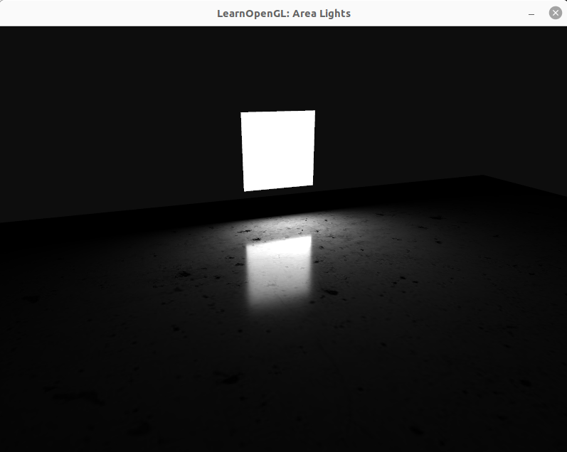
I also added a diffuse mapping of a concrete texture to the floor plane for a bit more realism. Provided you got all the code parts right you should be able to see something like this:

Measuring performance

This is all good and well, but you have probably wondered:

How can we place more area lights into a scene?
How fast/slow are the computations?

Obviously, both of these questions can have different answers depending on the graphics hardware, but in general it's pretty straight-forward to test: We can introduce a uniform array of area light sources to our shader, and we can use OpenGL timestamp queries for benchmarking. This is an interesting case since area lights require a lot of computation - significantly more than other types of light. So while we could probably fit 100-200 point lights in a scene and still have acceptable frame rates with plain forward rendering, this is not doable for area lights. So creating a lighting budget would be good advice if you want to release a game. The general setup for timestamp queries is shown below:

GLuint timeQuery;
glGenQueries(1, &timeQuery);

GLuint64 totalQueryTimeNs = 0;
GLuint64 numQueries = 0;

while (!glfwWindowShouldClose(window))
{
    [...]

    glBeginQuery(GL_TIME_ELAPSED, timeQuery);
    renderPlane();
    glEndQuery(GL_TIME_ELAPSED);

    GLuint64 elapsed = 0; // will be in nanoseconds
    glGetQueryObjectui64v(timeQuery, GL_QUERY_RESULT, &elapsed);
    numQueries++;
    totalQueryTimeNs += elapsed;
}

double measuredAverageNs = (double)totalQueryTimeNs / (double)numQueries;
double measuredAverageMs = measuredAverageNs * 1.0e-6;
std::cout << "Total average time(ms) = " << measuredAverageMs << '\n';

It is quite rudimentary, and does not take into account outliers or variance. The important part is the conversion from nanoseconds to milliseconds.

The fragment shader will use a loop to iterate over the lights. But we can reuse some of the information, e.g. we do not need to perform LUT texture lookups for each light. The changed parts of the fragment shader now looks like this:

struct AreaLight
{
    float intensity;
    vec3 color;
    vec3 points[4];
    bool twoSided;
};
uniform AreaLight areaLights[16];
uniform int numAreaLights;

// [...]

void main() {
    // [...]
    for (int i = 0; i < numAreaLights; i++)
    {
        // Evaluate LTC shading
        vec3 diffuse = LTC_Evaluate(N, V, P, mat3(1), areaLights[i].points, areaLights[i].twoSided);
        vec3 specular = LTC_Evaluate(N, V, P, Minv, areaLights[i].points, areaLights[i].twoSided);

        // GGX BRDF shadowing and Fresnel
        specular *= mSpecular*t2.x + (1.0f - mSpecular) * t2.y;

        // Add contribution
        result += areaLights[i].color * areaLights[i].intensity * (specular + mDiffuse * diffuse);
    }

    fragColor = vec4(ToSRGB(result), 1.0f);
}

We must specify a fixed length of the uniform array in OpenGL, even though in practice we will have fewer elements. So we set numAreaLights to a number equal to or less than the maximal allowed number of light sources, in our case 16.

The application can be constructed in many different ways, depending on your requirements. The important part is to create an array of area light positions and send them to the shader as uniforms. How this can be achieved was discussed in the chapter on Multiple lights. I shall here perform a rudimentary benchmark, as well as make some notes about the implementation:

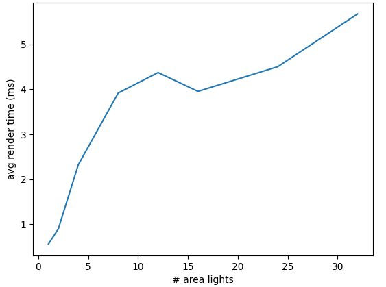
# area lights	Avg. rendering time (ms)
1	0.557326
2	0.897486
4	2.32212
8	3.9175
12	4.37243
16	3.95511
24	4.50246
32	5.67573

You may have a look at the source code, as well as the modified fragment shader.

Notes

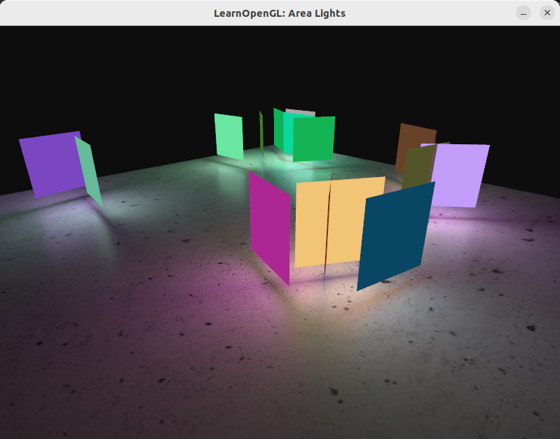
While this is not the most impressive demonstration, there are a few remarks and observations that can be made from this:

The lights are pseudo-randomly placed around the textured plane.
These measurements were made on a "NVIDIA GeForce GTX 850M" laptop GPU from 2015. You would likely (hopefully) experience better running times.
These lights were rendered with forward rendering.
I experienced a lot of variance when performing these benchmarks. And there are many factors to consider, like what the driver is doing, what other actions the program is performing, etc. The graph shows the general trend, which is a somewhat linear growth.
The numbers are obtained by wrapping the shader call which draws the textured plane with calls to glBeginQuery/glEndQuery, with the GL_TIME_ELAPSED target parameter. This query result may be obtained with glGetQueryObjectui64v and converted from nanoseconds to milliseconds for computing the desired average.

Especially the bullet about forward rendering is of particular interest here: In this scenario I have a single draw call, which is the textured plane (ignoring the colored planes that show the light sources). This setup is very unoptimal if you are rendering many objects, ie. computing the lighting contribution of each light source, for each fragment, for each mesh, as this would cause a lot of fragments to be discarded by depth testing.
A much better approach would be to use deferred lighting, which would mean computing the lighting per-fragment, regardless of the number of objects being drawn.

It is probably also possible to dispatch a compute shader which divides the screen area into tiles, and assigns a list of contributing area lights for each tile (ie. forward+ rendering), for further optimization. This would only work well if we could define a certain maximum attenuation radius for each area light, which e.g. has been done in Unreal engine (see Rectangular Area Lights).

Additional light types

It is possible to implement other types of area light sources, such as line lights or cylinder lights. Albeit out-of-scope for this article, the mathematical foundation may be found in [12]. I have not tried to implement these myself, and thus cannot speak for their efficiency or implementation details. They are simply included here for completeness. I have also observed some presentations that include circular area lights.

Conclusion

Thank you for reading. I hope you enjoyed and learned something. For myself it was an immense pleasure learning about this awesome technique, and all credits go to the researchers who discovered it. As mentioned in the beginning, later extensions were made to this technique, including other types of light polygons. These, as well as a section on texture mapping was omitted from this tutorial for reasons of brevity. They might, however, be touched upon in a future chapter.

As an ending note, it’s worth mentioning that adding shadows to area light sources is an open research field. Some possible ideas involve screen-space raytracing with statistical denoising, such as [9] or [10]. While obviously very interesting, these techniques are a bit out-of-scope for this tutorial series. You may of course investigate further, if you wish.

Article by: Alexander Christensen

References

[1] Real-Time Polygonal-Light Shading with Linearly Transformed Cosines, ACM Siggraph '16, LTC.pdf
[2] Real-Time Area Lighting: a Journey from Research to Production, presentation slides by Stephen Hill: s2016_ltc_rnd.pdf
[3] Real-Time Polygonal-Light Shading with Linearly Transformed Cosines, presentationslides by Eric Heitz: slides.pdf
[4] Main reference github repo: https://github.com/selfshadow/ltc_code. Contains precomputed matrices, source code for WebGL examples, and source code for recomputing the matrices with different BRDF-models.
[5] Lighting with Linearly Transformed Cosines, blog post by Tom Grove further investigating the technique. blog
[6] Real-Time Polygonal-Light Shading with Linearly Transformed Cosines, Supplemental video showcasing the technique: Youtube
[7] Adam - Unity, award-winning real-time-rendered short film by the Unity Demo team using the technique: Youtube
[8] Interactive WebGL-demo: blog.selfshadow.com
[9] Combining Analytic Direct Illumination and Stochastic Shadows, Eric Heitz et al.: I3D2018 combining.pdf
[10] Fast Analytic Soft Shadows from Area Lights, Aakash KT et al.: 111-120.pdf
[11] Stoke's theorem: Wikipedia
[12] Linear-Light Shading with Linearly Transformed Cosines: HAL archives
[13] Alan Watt and Mark Watt: Advanced Animation and Rendering Techniques, Theory and Practice, Addison Wesley, 1992