


Lighting
PBR/Lighting
In the previous chapter we laid the foundation for getting a realistic physically based renderer off the ground. In this chapter we'll focus on translating the previously discussed theory into an actual renderer that uses direct (or analytic) light sources: think of point lights, directional lights, and/or spotlights.
Let's start by re-visiting the final reflectance equation from the previous chapter:
\[ L_o(p,\omega_o) = \int\limits_{\Omega} (k_d\frac{c}{\pi} + \frac{DFG}{4(\omega_o \cdot n)(\omega_i \cdot n)}) L_i(p,\omega_i) n \cdot \omega_i d\omega_i \]We now know mostly what's going on, but what still remained a big unknown is how exactly we're going to represent irradiance, the total radiance \(L\), of the scene. We know that radiance \(L\) (as interpreted in computer graphics land) measures the radiant flux \(\phi\) or light energy of a light source over a given solid angle \(\omega\). In our case we assumed the solid angle \(\omega\) to be infinitely small in which case radiance measures the flux of a light source over a single light ray or direction vector.
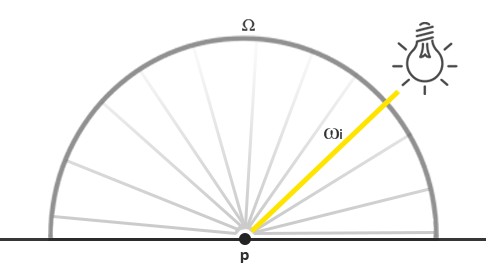
Given this knowledge, how do we translate this into some of the lighting knowledge we've accumulated from previous chapters? Well, imagine we have a single point light (a light source that shines equally bright in all directions) with a radiant flux of (23.47, 21.31, 20.79) as translated to an RGB triplet. The radiant intensity of this light source equals its radiant flux at all outgoing direction rays. However, when shading a specific point \(p\) on a surface, of all possible incoming light directions over its hemisphere \(\Omega\), only one incoming direction vector \(w_i\) directly comes from the point light source. As we only have a single light source in our scene, assumed to be a single point in space, all other possible incoming light directions have zero radiance observed over the surface point \(p\):
If at first, we assume that light attenuation (dimming of light over distance) does not affect the point light source, the radiance of the incoming light ray is the same regardless of where we position the light (excluding scaling the radiance by the incident angle \(\cos \theta\)). This, because the point light has the same radiant intensity regardless of the angle we look at it, effectively modeling its radiant intensity as its radiant flux: a constant vector (23.47, 21.31, 20.79).
However, radiance also takes a position \(p\) as input and as any realistic point light source takes light attenuation into account, the radiant intensity of the point light source is scaled by some measure of the distance between point \(p\) and the light source. Then, as extracted from the original radiance equation, the result is scaled by the dot product between the surface normal \(n\) and the incoming light direction \(w_i\).
To put this in more practical terms: in the case of a direct point light the radiance function \(L\) measures the light color, attenuated over its distance to \(p\) and scaled by \(n \cdot w_i\), but only over the single light ray \(w_i\) that hits \(p\) which equals the light's direction vector from \(p\). In code this translates to:
vec3  lightColor  = vec3(23.47, 21.31, 20.79);
vec3  wi          = normalize(lightPos - fragPos);
float cosTheta    = max(dot(N, Wi), 0.0);
float attenuation = calculateAttenuation(fragPos, lightPos);
vec3  radiance    = lightColor * attenuation * cosTheta;
Aside from the different terminology, this piece of code should be awfully familiar to you: this is exactly how we've been doing diffuse lighting so far. When it comes to direct lighting, radiance is calculated similarly to how we've calculated lighting before as only a single light direction vector contributes to the surface's radiance.
For other types of light sources originating from a single point we calculate radiance similarly. For instance, a directional light source has a constant \(w_i\) without an attenuation factor. And a spotlight would not have a constant radiant intensity, but one that is scaled by the forward direction vector of the spotlight.
This also brings us back to the integral \(\int\) over the surface's hemisphere \(\Omega\) . As we know beforehand the single locations of all the contributing light sources while shading a single surface point, it is not required to try and solve the integral. We can directly take the (known) number of light sources and calculate their total irradiance, given that each light source has only a single light direction that influences the surface's radiance. This makes PBR on direct light sources relatively simple as we effectively only have to loop over the contributing light sources. When we later take environment lighting into account in the IBL chapters we do have to take the integral into account as light can come from any direction.
A PBR surface model
Let's start by writing a fragment shader that implements the previously described PBR models. First, we need to take the relevant PBR inputs required for shading the surface:
#version 330 core
out vec4 FragColor;
in vec2 TexCoords;
in vec3 WorldPos;
in vec3 Normal;

uniform vec3 camPos;

uniform vec3  albedo;
uniform float metallic;
uniform float roughness;
uniform float ao;
We take the standard inputs as calculated from a generic vertex shader and a set of constant material properties over the surface of the object.
Then at the start of the fragment shader we do the usual calculations required for any lighting algorithm:
void main()
{
    vec3 N = normalize(Normal);
    vec3 V = normalize(camPos - WorldPos);
    [...]
}
Direct lighting
In this chapter's example demo we have a total of 4 point lights that together represent the scene's irradiance. To satisfy the reflectance equation we loop over each light source, calculate its individual radiance and sum its contribution scaled by the BRDF and the light's incident angle. We can think of the loop as solving the integral \(\int\) over \(\Omega\) for direct light sources. First, we calculate the relevant per-light variables:
vec3 Lo = vec3(0.0);
for(int i = 0; i < 4; ++i)
{
    vec3 L = normalize(lightPositions[i] - WorldPos);
    vec3 H = normalize(V + L);

    float distance    = length(lightPositions[i] - WorldPos);
    float attenuation = 1.0 / (distance * distance);
    vec3 radiance     = lightColors[i] * attenuation;
    [...]
As we calculate lighting in linear space (we'll gamma correct at the end of the shader) we attenuate the light sources by the more physically correct
Then, for each light we want to calculate the full Cook-Torrance specular BRDF term:
\[ \frac{DFG}{4(\omega_o \cdot n)(\omega_i \cdot n)} \]
The first thing we want to do is calculate the ratio between specular and diffuse reflection, or how much the surface reflects light versus how much it refracts light. We know from the previous chapter that the Fresnel equation calculates just that (note the clamp here to prevent black spots):
vec3 fresnelSchlick(float cosTheta, vec3 F0)
{
    return F0 + (1.0 - F0) * pow(clamp(1.0 - cosTheta, 0.0, 1.0), 5.0);
}
The Fresnel-Schlick approximation expects a F0 parameter which is known as the surface reflection at zero incidence or how much the surface reflects if looking directly at the surface. The F0 varies per material and is tinted on metals as we find in large material databases. In the PBR metallic workflow we make the simplifying assumption that most dielectric surfaces look visually correct with a constant F0 of 0.04, while we do specify F0 for metallic surfaces as then given by the albedo value. This translates to code as follows:
vec3 F0 = vec3(0.04);
F0      = mix(F0, albedo, metallic);
vec3 F  = fresnelSchlick(max(dot(H, V), 0.0), F0);
As you can see, for non-metallic surfaces F0 is always 0.04. For metallic surfaces, we vary F0 by linearly interpolating between the original F0 and the albedo value given the metallic property.
Given \(F\), the remaining terms to calculate are the normal distribution function \(D\) and the geometry function \(G\).
In a direct PBR lighting shader their code equivalents are:
float DistributionGGX(vec3 N, vec3 H, float roughness)
{
    float a      = roughness*roughness;
    float a2     = a*a;
    float NdotH  = max(dot(N, H), 0.0);
    float NdotH2 = NdotH*NdotH;

    float num   = a2;
    float denom = (NdotH2 * (a2 - 1.0) + 1.0);
    denom = PI * denom * denom;

    return num / denom;
}

float GeometrySchlickGGX(float NdotV, float roughness)
{
    float r = (roughness + 1.0);
    float k = (r*r) / 8.0;

    float num   = NdotV;
    float denom = NdotV * (1.0 - k) + k;

    return num / denom;
}
float GeometrySmith(vec3 N, vec3 V, vec3 L, float roughness)
{
    float NdotV = max(dot(N, V), 0.0);
    float NdotL = max(dot(N, L), 0.0);
    float ggx2  = GeometrySchlickGGX(NdotV, roughness);
    float ggx1  = GeometrySchlickGGX(NdotL, roughness);

    return ggx1 * ggx2;
}
What's important to note here is that in contrast to the theory chapter, we pass the roughness parameter directly to these functions; this way we can make some term-specific modifications to the original roughness value. Based on observations by Disney and adopted by Epic Games, the lighting looks more correct squaring the roughness in both the geometry and normal distribution function.
With both functions defined, calculating the NDF and the G term in the reflectance loop is straightforward:
float NDF = DistributionGGX(N, H, roughness);
float G   = GeometrySmith(N, V, L, roughness);
This gives us enough to calculate the Cook-Torrance BRDF:
vec3 numerator    = NDF * G * F;
float denominator = 4.0 * max(dot(N, V), 0.0) * max(dot(N, L), 0.0)  + 0.0001;
vec3 specular     = numerator / denominator;
Note that we add 0.0001 to the denominator to prevent a divide by zero in case any dot product ends up 0.0.
Now we can finally calculate each light's contribution to the reflectance equation. As the Fresnel value directly corresponds to \(k_S\) we can use F to denote the specular contribution of any light that hits the surface. From \(k_S\) we can then calculate the ratio of refraction \(k_D\):
vec3 kS = F;
vec3 kD = vec3(1.0) - kS;

kD *= 1.0 - metallic;
Seeing as kS represents the energy of light that gets reflected, the remaining ratio of light energy is the light that gets refracted which we store as kD. Furthermore, because metallic surfaces don't refract light and thus have no diffuse reflections we enforce this property by nullifying kD if the surface is metallic. This gives us the final data we need to calculate each light's outgoing reflectance value:
    const float PI = 3.14159265359;

    float NdotL = max(dot(N, L), 0.0);
    Lo += (kD * albedo / PI + specular) * radiance * NdotL;
}
The resulting Lo value, or the outgoing radiance, is effectively the result of the reflectance equation's integral \(\int\) over \(\Omega\). We don't really have to try and solve the integral for all possible incoming light directions as we know exactly the 4 incoming light directions that can influence the fragment. Because of this, we can directly loop over these incoming light directions e.g. the number of lights in the scene.
What's left is to add an (improvised) ambient term to the direct lighting result Lo and we have the final lit color of the fragment:
vec3 ambient = vec3(0.03) * albedo * ao;
vec3 color   = ambient + Lo;
Linear and HDR rendering
So far we've assumed all our calculations to be in linear color space and to account for this we need to gamma correct at the end of the shader. Calculating lighting in linear space is incredibly important as PBR requires all inputs to be linear. Not taking this into account will result in incorrect lighting. Additionally, we want light inputs to be close to their physical equivalents such that their radiance or color values can vary wildly over a high spectrum of values. As a result, Lo can rapidly grow really high which then gets clamped between 0.0 and 1.0 due to the default low dynamic range (LDR) output. We fix this by taking Lo and tone or exposure map the high dynamic range (HDR) value correctly to LDR before gamma correction:
color = color / (color + vec3(1.0));
color = pow(color, vec3(1.0/2.2));
Here we tone map the HDR color using the Reinhard operator, preserving the high dynamic range of a possibly highly varying irradiance, after which we gamma correct the color. We don't have a separate framebuffer or post-processing stage so we can directly apply both the tone mapping and gamma correction step at the end of the forward fragment shader.
Taking both linear color space and high dynamic range into account is incredibly important in a PBR pipeline. Without these it's impossible to properly capture the high and low details of varying light intensities and your calculations end up incorrect and thus visually unpleasing.
Full direct lighting PBR shader
All that's left now is to pass the final tone mapped and gamma corrected color to the fragment shader's output channel and we have ourselves a direct PBR lighting shader. For completeness' sake, the complete
#version 330 core
out vec4 FragColor;
in vec2 TexCoords;
in vec3 WorldPos;
in vec3 Normal;

// material parameters
uniform vec3  albedo;
uniform float metallic;
uniform float roughness;
uniform float ao;

// lights
uniform vec3 lightPositions[4];
uniform vec3 lightColors[4];

uniform vec3 camPos;

const float PI = 3.14159265359;

float DistributionGGX(vec3 N, vec3 H, float roughness);
float GeometrySchlickGGX(float NdotV, float roughness);
float GeometrySmith(vec3 N, vec3 V, vec3 L, float roughness);
vec3 fresnelSchlick(float cosTheta, vec3 F0);

void main()
{
    vec3 N = normalize(Normal);
    vec3 V = normalize(camPos - WorldPos);

    vec3 F0 = vec3(0.04);
    F0 = mix(F0, albedo, metallic);

    // reflectance equation
    vec3 Lo = vec3(0.0);
    for(int i = 0; i < 4; ++i)
    {
        // calculate per-light radiance
        vec3 L = normalize(lightPositions[i] - WorldPos);
        vec3 H = normalize(V + L);
        float distance    = length(lightPositions[i] - WorldPos);
        float attenuation = 1.0 / (distance * distance);
        vec3 radiance     = lightColors[i] * attenuation;

        // cook-torrance brdf
        float NDF = DistributionGGX(N, H, roughness);
        float G   = GeometrySmith(N, V, L, roughness);
        vec3 F    = fresnelSchlick(max(dot(H, V), 0.0), F0);

        vec3 kS = F;
        vec3 kD = vec3(1.0) - kS;
        kD *= 1.0 - metallic;

        vec3 numerator    = NDF * G * F;
        float denominator = 4.0 * max(dot(N, V), 0.0) * max(dot(N, L), 0.0) + 0.0001;
        vec3 specular     = numerator / denominator;

        // add to outgoing radiance Lo
        float NdotL = max(dot(N, L), 0.0);
        Lo += (kD * albedo / PI + specular) * radiance * NdotL;
    }

    vec3 ambient = vec3(0.03) * albedo * ao;
    vec3 color = ambient + Lo;

    color = color / (color + vec3(1.0));
    color = pow(color, vec3(1.0/2.2));

    FragColor = vec4(color, 1.0);
}
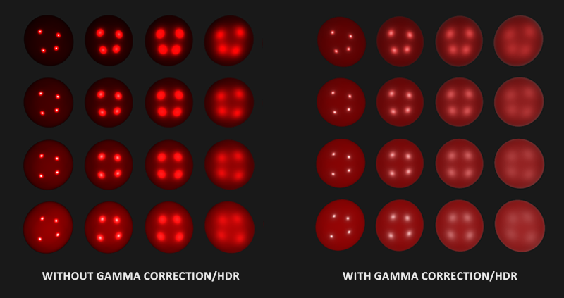
Hopefully, with the theory from the previous chapter and the knowledge of the reflectance equation this shader shouldn't be as daunting anymore. If we take this shader, 4 point lights, and quite a few spheres where we vary both their metallic and roughness values on their vertical and horizontal axis respectively, we'd get something like this:
From bottom to top the metallic value ranges from 0.0 to 1.0, with roughness increasing left to right from 0.0 to 1.0. You can see that by only changing these two simple to understand parameters we can already display a wide array of different materials.
You can find the full source code of the demo here.
Textured PBR
Extending the system to now accept its surface parameters as textures instead of uniform values gives us per-fragment control over the surface material's properties:
[...]
uniform sampler2D albedoMap;
uniform sampler2D normalMap;
uniform sampler2D metallicMap;
uniform sampler2D roughnessMap;
uniform sampler2D aoMap;

void main()
{
    vec3 albedo     = pow(texture(albedoMap, TexCoords).rgb, 2.2);
    vec3 normal     = getNormalFromNormalMap();
    float metallic  = texture(metallicMap, TexCoords).r;
    float roughness = texture(roughnessMap, TexCoords).r;
    float ao        = texture(aoMap, TexCoords).r;
    [...]
}
Note that the albedo textures that come from artists are generally authored in sRGB space which is why we first convert them to linear space before using albedo in our lighting calculations. Based on the system artists use to generate ambient occlusion maps you may also have to convert these from sRGB to linear space as well. Metallic and roughness maps are almost always authored in linear space.
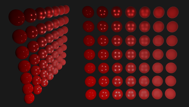
Replacing the material properties of the previous set of spheres with textures, already shows a major visual improvement over the previous lighting algorithms we've used:
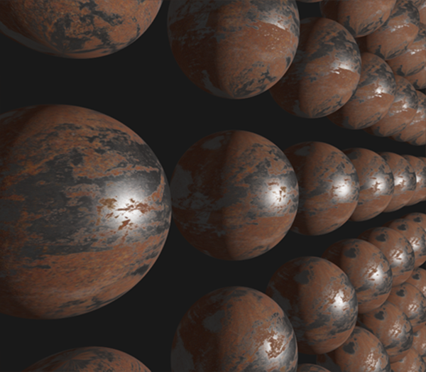
You can find the full source code of the textured demo here and the texture set used here (with a white ao map). Keep in mind that metallic surfaces tend to look too dark in direct lighting environments as they don't have diffuse reflectance. They do look more correct when taking the environment's specular ambient lighting into account, which is what we'll focus on in the next chapters.
While not as visually impressive as some of the PBR render demos you find out there, given that we don't yet have image based lighting built in, the system we have now is still a physically based renderer, and even without IBL you'll see your lighting look a lot more realistic.