


Theory
PBR/Theory
PBR, or more commonly known as
Physically based rendering is still nonetheless an approximation of reality (based on the principles of physics) which is why it's not called physical shading, but physically based shading. For a PBR lighting model to be considered physically based, it has to satisfy the following 3 conditions (don't worry, we'll get to them soon enough):
- Be based on the microfacet surface model.
- Be energy conserving.
- Use a physically based BRDF.
In the next PBR chapters we'll be focusing on the PBR approach as originally explored by Disney and adopted for real-time display by Epic Games. Their approach, based on the
Keep in mind, the topics in these chapters are rather advanced so it is advised to have a good understanding of OpenGL and shader lighting. Some of the more advanced knowledge you'll need for this series are: framebuffers, cubemaps, gamma correction, HDR, and normal mapping. We'll also delve into some advanced mathematics, but I'll do my best to explain the concepts as clear as possible.
The microfacet model
All the PBR techniques are based on the theory of microfacets. The theory describes that any surface at a microscopic scale can be described by tiny little perfectly reflective mirrors called

The rougher a surface is, the more chaotically aligned each microfacet will be along the surface. The effect of these tiny-like mirror alignments is, that when specifically talking about specular lighting/reflection, the incoming light rays are more likely to

No surface is completely smooth on a microscopic level, but seeing as these microfacets are small enough that we can't make a distinction between them on a per-pixel basis, we statistically approximate the surface's microfacet roughness given a
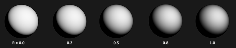
The more the microfacets are aligned to the halfway vector, the sharper and stronger the specular reflection. Together with a roughness parameter that varies between 0 and 1, we can statistically approximate the alignment of the microfacets:
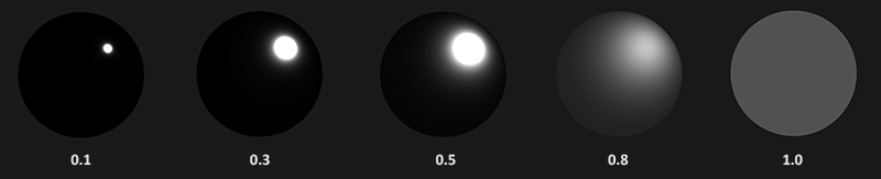
We can see that higher roughness values display a much larger specular reflection shape, in contrast with the smaller and sharper specular reflection shape of smooth surfaces.
Energy conservation
The microfacet approximation employs a form of
For energy conservation to hold, we need to make a clear distinction between diffuse and specular light. The moment a light ray hits a surface, it gets split in both a
There are some nuances here as refracted light doesn't immediately get absorbed by touching the surface. From physics, we know that light can be modeled as a beam of energy that keeps moving forward until it loses all of its energy; the way a light beam loses energy is by collision. Each material consists of tiny little particles that can collide with the light ray as illustrated in the following image. The particles absorb some, or all, of the light's energy at each collision which is converted into heat.
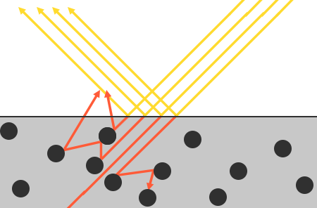
Generally, not all energy is absorbed and the light will continue to
An additional subtlety when it comes to reflection and refraction are surfaces that are
This distinction between reflected and refracted light brings us to another observation regarding energy preservation: they're mutually exclusive. Whatever light energy gets reflected will no longer be absorbed by the material itself. Thus, the energy left to enter the surface as refracted light is directly the resulting energy after we've taken reflection into account.
We preserve this energy conserving relation by first calculating the specular fraction that amounts the percentage the incoming light's energy is reflected. The fraction of refracted light is then directly calculated from the specular fraction as:
float kS = calculateSpecularComponent(...); // reflection/specular fraction
float kD = 1.0 - kS;                        // refraction/diffuse  fraction
This way we know both the amount the incoming light reflects and the amount the incoming light refracts, while adhering to the energy conservation principle. Given this approach, it is impossible for both the refracted/diffuse and reflected/specular contribution to exceed 1.0, thus ensuring the sum of their energy never exceeds the incoming light energy. Something we did not take into account in the previous lighting chapters.
The reflectance equation
This brings us to something called the render equation, an elaborate equation some very smart folks out there came up with that is currently the best model we have for simulating the visuals of light. Physically based rendering strongly follows a more specialized version of the render equation known as the
The reflectance equation appears daunting at first, but as we'll dissect it you'll see it slowly starts to makes sense. To understand the equation, we have to delve into a bit of
Radiant flux: radiant flux \(\Phi\) is the transmitted energy of a light source measured in Watts. Light is a collective sum of energy over multiple different wavelengths, each wavelength associated with a particular (visible) color. The emitted energy of a light source can therefore be thought of as a function of all its different wavelengths. Wavelengths between 390nm to 700nm (nanometers) are considered part of the visible light spectrum i.e. wavelengths the human eye is able to perceive. Below you'll find an image of the different energies per wavelength of daylight:
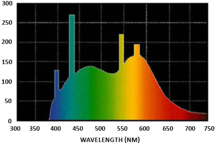
The radiant flux measures the total area of this function of different wavelengths. Directly taking this measure of wavelengths as input is slightly impractical so we often make the simplification of representing radiant flux, not as a function of varying wavelength strengths, but as a light color triplet encoded as RGB (or as we'd commonly call it: light color). This encoding does come at quite a loss of information, but this is generally negligible for visual aspects.
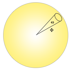
Solid angle: the solid angle, denoted as \(\omega\), tells us the size or area of a shape projected onto a unit sphere. The area of the projected shape onto this unit sphere is known as the

Think of being an observer at the center of this unit sphere and looking in the direction of the shape; the size of the silhouette you make out of it is the solid angle.
Radiant intensity: radiant intensity measures the amount of radiant flux per solid angle, or the strength of a light source over a projected area onto the unit sphere. For instance, given an omnidirectional light that radiates equally in all directions, the radiant intensity can give us its energy over a specific area (solid angle):
The equation to describe the radiant intensity is defined as follows:
\[I = \frac{d\Phi}{d\omega}\]Where \(I\) is the radiant flux \(\Phi\) over the solid angle \(\omega\).
With knowledge of radiant flux, radiant intensity, and the solid angle, we can finally describe the equation for radiance. Radiance is described as the total observed energy in an area \(A\) over the solid angle \(\omega\) of a light of radiant intensity \(\Phi\):
\[L=\frac{d^2\Phi}{ dA d\omega \cos\theta}\]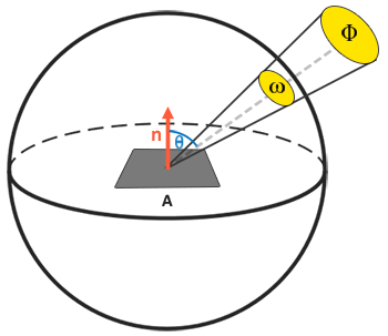
Radiance is a radiometric measure of the amount of light in an area, scaled by the
float cosTheta = dot(lightDir, N);
The radiance equation is quite useful as it contains most physical quantities we're interested in. If we consider the solid angle \(\omega\) and the area \(A\) to be infinitely small, we can use radiance to measure the flux of a single ray of light hitting a single point in space. This relation allows us to calculate the radiance of a single light ray influencing a single (fragment) point; we effectively translate the solid angle \(\omega\) into a direction vector \(\omega\), and \(A\) into a point \(p\). This way, we can directly use radiance in our shaders to calculate a single light ray's per-fragment contribution.
In fact, when it comes to radiance we generally care about all incoming light onto a point \(p\), which is the sum of all radiance known as
We now know that \(L\) in the render equation represents the radiance of some point \(p\) and some incoming infinitely small solid angle \(\omega_i\) which can be thought of as an incoming direction vector \(\omega_i\). Remember that \(\cos \theta\) scales the energy based on the light's incident angle to the surface, which we find in the reflectance equation as \(n \cdot \omega_i\). The reflectance equation calculates the sum of reflected radiance \(L_o(p, \omega_o)\) of a point \(p\) in direction \(\omega_o\) which is the outgoing direction to the viewer. Or to put it differently: \(L_o\) measures the reflected sum of the lights' irradiance onto point \(p\) as viewed from \(\omega_o\).
The reflectance equation is based around irradiance, which is the sum of all incoming radiance we measure light of. Not just of a single incoming light direction, but of all incoming light directions within a hemisphere \(\Omega\) centered around point \(p\). A

To calculate the total of values inside an area or (in the case of a hemisphere) a volume, we use a mathematical construct called an
int steps = 100;
float sum = 0.0f;
vec3 P    = ...;
vec3 Wo   = ...;
vec3 N    = ...;
float dW  = 1.0f / steps;
for(int i = 0; i < steps; ++i)
{
    vec3 Wi = getNextIncomingLightDir(i);
    sum += Fr(P, Wi, Wo) * L(P, Wi) * dot(N, Wi) * dW;
}
By scaling the steps by dW, the sum will equal the total area or volume of the integral function. The dW to scale each discrete step can be thought of as \(d\omega_i\) in the reflectance equation. Mathematically \(d\omega_i\) is the continuous symbol over which we calculate the integral, and while it does not directly relate to dW in code (as this is a discrete step of the Riemann sum), it helps to think of it this way. Keep in mind that taking discrete steps will always give us an approximation of the total area of the function. A careful reader will notice we can increase the accuracy of the Riemann Sum by increasing the number of steps.
The reflectance equation sums up the radiance of all incoming light directions \(\omega_i\) over the hemisphere \(\Omega\) scaled by \(f_r\) that hit point \(p\) and returns the sum of reflected light \(L_o\) in the viewer's direction. The incoming radiance can come from light sources as we're familiar with, or from an environment map measuring the radiance of every incoming direction as we'll discuss in the IBL chapters.
Now the only unknown left is the \(f_r\) symbol known as the
BRDF
The
A BRDF approximates the material's reflective and refractive properties based on the previously discussed microfacet theory. For a BRDF to be physically plausible it has to respect the law of energy conservation i.e. the sum of reflected light should never exceed the amount of incoming light. Technically, Blinn-Phong is considered a BRDF taking the same \(\omega_i\) and \(\omega_o\) as inputs. However, Blinn-Phong is not considered physically based as it doesn't adhere to the energy conservation principle. There are several physically based BRDFs out there to approximate the surface's reaction to light. However, almost all real-time PBR render pipelines use a BRDF known as the
The Cook-Torrance BRDF contains both a diffuse and specular part:
\[f_r = k_d f_{lambert} + k_s f_{cook-torrance}\]
Here \(k_d\) is the earlier mentioned ratio of incoming light energy that gets refracted with \(k_s\) being the ratio that gets reflected. The left side of the BRDF states the diffuse part of the equation denoted here as \(f_{lambert}\). This is known as
With \(c\) being the albedo or surface color (think of the diffuse surface texture). The divide by pi is there to normalize the diffuse light as the earlier denoted integral that contains the BRDF is scaled by \(\pi\) (we'll get to that in the IBL chapters).
There exist different equations for the diffuse part of the BRDF which tend to look more realistic, but are also more computationally expensive. As concluded by Epic Games however, the Lambertian diffuse is sufficient enough for most real-time rendering purposes.
The specular part of the BRDF is a bit more advanced and is described as:
\[ f_{CookTorrance} = \frac{DFG}{4(\omega_o \cdot n)(\omega_i \cdot n)} \]The Cook-Torrance specular BRDF is composed three functions and a normalization factor in the denominator. Each of the D, F and G symbols represent a type of function that approximates a specific part of the surface's reflective properties. These are defined as the normal Distribution function, the Fresnel equation and the Geometry function:
- Normal distribution function: approximates the amount the surface's microfacets are aligned to the halfway vector, influenced by the roughness of the surface; this is the primary function approximating the microfacets.
- Geometry function: describes the self-shadowing property of the microfacets. When a surface is relatively rough, the surface's microfacets can overshadow other microfacets reducing the light the surface reflects.
- Fresnel equation: The Fresnel equation describes the ratio of surface reflection at different surface angles.
Each of these functions are an approximation of their physics equivalents and you'll find more than one version of each that aims to approximate the underlying physics in different ways; some more realistic, others more efficient. It is perfectly fine to pick whatever approximated version of these functions you want to use. Brian Karis from Epic Games did a great deal of research on the multiple types of approximations here. We're going to pick the same functions used by Epic Game's Unreal Engine 4 which are the Trowbridge-Reitz GGX for D, the Fresnel-Schlick approximation for F, and the Smith's Schlick-GGX for G.
Normal distribution function
The
Here \(h\) is the halfway vector to measure against the surface's microfacets, with \(a\) being a measure of the surface's roughness. If we take \(h\) as the halfway vector between the surface normal and light direction over varying roughness parameters we get the following visual result:
When the roughness is low (thus the surface is smooth), a highly concentrated number of microfacets are aligned to halfway vectors over a small radius. Due to this high concentration, the NDF displays a very bright spot. On a rough surface however, where the microfacets are aligned in much more random directions, you'll find a much larger number of halfway vectors \(h\) somewhat aligned to the microfacets (but less concentrated), giving us the more grayish results.
In GLSL the Trowbridge-Reitz GGX normal distribution function translates to the following code:
float DistributionGGX(vec3 N, vec3 H, float a)
{
    float a2     = a*a;
    float NdotH  = max(dot(N, H), 0.0);
    float NdotH2 = NdotH*NdotH;

    float nom    = a2;
    float denom  = (NdotH2 * (a2 - 1.0) + 1.0);
    denom        = PI * denom * denom;

    return nom / denom;
}
Geometry function
The geometry function statistically approximates the relative surface area where its micro surface-details overshadow each other, causing light rays to be occluded.

Similar to the NDF, the Geometry function takes a material's roughness parameter as input with rougher surfaces having a higher probability of overshadowing microfacets. The geometry function we will use is a combination of the GGX and Schlick-Beckmann approximation known as Schlick-GGX:
\[ G_{SchlickGGX}(n, v, k) = \frac{n \cdot v} {(n \cdot v)(1 - k) + k } \]Here \(k\) is a remapping of \(\alpha\) based on whether we're using the geometry function for either direct lighting or IBL lighting:
\[ k_{direct} = \frac{(\alpha + 1)^2}{8} \] \[ k_{IBL} = \frac{\alpha^2}{2} \]Note that the value of \(\alpha\) may differ based on how your engine translates roughness to \(\alpha\). In the following chapters we'll extensively discuss how and where this remapping becomes relevant.
To effectively approximate the geometry we need to take account of both the view direction (geometry obstruction) and the light direction vector (geometry shadowing). We can take both into account using
Using Smith's method with Schlick-GGX as \(G_{sub}\) gives the following visual appearance over varying roughness R:
The geometry function is a multiplier between [0.0, 1.0] with 1.0 (or white) measuring no microfacet shadowing, and 0.0 (or black) complete microfacet shadowing.
In GLSL the geometry function translates to the following code:
float GeometrySchlickGGX(float NdotV, float k)
{
    float nom   = NdotV;
    float denom = NdotV * (1.0 - k) + k;

    return nom / denom;
}

float GeometrySmith(vec3 N, vec3 V, vec3 L, float k)
{
    float NdotV = max(dot(N, V), 0.0);
    float NdotL = max(dot(N, L), 0.0);
    float ggx1 = GeometrySchlickGGX(NdotV, k);
    float ggx2 = GeometrySchlickGGX(NdotL, k);

    return ggx1 * ggx2;
}
Fresnel equation
The Fresnel equation (pronounced as Freh-nel) describes the ratio of light that gets reflected over the light that gets refracted, which varies over the angle we're looking at a surface. The moment light hits a surface, based on the surface-to-view angle, the Fresnel equation tells us the percentage of light that gets reflected. From this ratio of reflection and the energy conservation principle we can directly obtain the refracted portion of light.
Every surface or material has a level of
The Fresnel equation is a rather complex equation, but luckily the Fresnel equation can be approximated using the
\(F_0\) represents the base reflectivity of the surface, which we calculate using something called the indices of refraction or IOR. As you can see on a sphere surface, the more we look towards the surface's grazing angles (with the halfway-view angle reaching 90 degrees), the stronger the Fresnel and thus the reflections:
There are a few subtleties involved with the Fresnel equation. One is that the Fresnel-Schlick approximation is only really defined for
The surface's response at normal incidence, or the base reflectivity, can be found in large databases like these with some of the more common values listed below as taken from Naty Hoffman's course notes:
| Material | \(F_0\) (Linear) | \(F_0\) (sRGB) | Color |
|---|---|---|---|
| Water | (0.02, 0.02, 0.02) |
(0.15, 0.15, 0.15) |
|
| Plastic / Glass (Low) | (0.03, 0.03, 0.03) |
(0.21, 0.21, 0.21) |
|
| Plastic High | (0.05, 0.05, 0.05) |
(0.24, 0.24, 0.24) |
|
| Glass (high) / Ruby | (0.08, 0.08, 0.08) |
(0.31, 0.31, 0.31) |
|
| Diamond | (0.17, 0.17, 0.17) |
(0.45, 0.45, 0.45) |
|
| Iron | (0.56, 0.57, 0.58) |
(0.77, 0.78, 0.78) |
|
| Copper | (0.95, 0.64, 0.54) |
(0.98, 0.82, 0.76) |
|
| Gold | (1.00, 0.71, 0.29) |
(1.00, 0.86, 0.57) |
|
| Aluminium | (0.91, 0.92, 0.92) |
(0.96, 0.96, 0.97) |
|
| Silver | (0.95, 0.93, 0.88) |
(0.98, 0.97, 0.95) |
What is interesting to observe here is that for all dielectric surfaces the base reflectivity never gets above 0.17 which is the exception rather than the rule, while for conductors the base reflectivity starts much higher and (mostly) varies between 0.5 and 1.0. Furthermore, for conductors (or metallic surfaces) the base reflectivity is tinted. This is why \(F_0\) is presented as an RGB triplet (reflectivity at normal incidence can vary per wavelength); this is something we only see at metallic surfaces.
These specific attributes of metallic surfaces compared to dielectric surfaces gave rise to something called the
By pre-computing \(F_0\) for both dielectrics and conductors we can use the same Fresnel-Schlick approximation for both types of surfaces, but we do have to tint the base reflectivity if we have a metallic surface. We generally accomplish this as follows:
vec3 F0 = vec3(0.04);
F0      = mix(F0, surfaceColor.rgb, metalness);
We define a base reflectivity that is approximated for most dielectric surfaces. This is yet another approximation as \(F_0\) is averaged around most common dielectrics. A base reflectivity of 0.04 holds for most dielectrics and produces physically plausible results without having to author an additional surface parameter. Then, based on how metallic a surface is, we either take the dielectric base reflectivity or take \(F_0\) authored as the surface color. Because metallic surfaces absorb all refracted light they have no diffuse reflections and we can directly use the surface color texture as their base reflectivity.
In code, the Fresnel Schlick approximation translates to:
vec3 fresnelSchlick(float cosTheta, vec3 F0)
{
    return F0 + (1.0 - F0) * pow(1.0 - cosTheta, 5.0);
}
With cosTheta being the dot product result between the surface's normal \(n\) and the halfway \(h\) (or view \(v\)) direction.
Cook-Torrance reflectance equation
With every component of the Cook-Torrance BRDF described, we can include the physically based BRDF into the now final reflectance equation:
\[ L_o(p,\omega_o) = \int\limits_{\Omega} (k_d\frac{c}{\pi} + k_s\frac{DFG}{4(\omega_o \cdot n)(\omega_i \cdot n)}) L_i(p,\omega_i) n \cdot \omega_i d\omega_i \]This equation is not fully mathematically correct however. You may remember that the Fresnel term \(F\) represents the ratio of light that gets reflected on a surface. This is effectively our ratio \(k_s\), meaning the specular (BRDF) part of the reflectance equation implicitly contains the reflectance ratio \(k_s\). Given this, our final final reflectance equation becomes:
\[ L_o(p,\omega_o) = \int\limits_{\Omega} (k_d\frac{c}{\pi} + \frac{DFG}{4(\omega_o \cdot n)(\omega_i \cdot n)}) L_i(p,\omega_i) n \cdot \omega_i d\omega_i \]This equation now completely describes a physically based render model that is generally recognized as what we commonly understand as physically based rendering, or PBR. Don't worry if you didn't yet completely understand how we'll need to fit all the discussed mathematics together in code. In the next chapters, we'll explore how to utilize the reflectance equation to get much more physically plausible results in our rendered lighting and all the bits and pieces should slowly start to fit together.
Authoring PBR materials
With knowledge of the underlying mathematical model of PBR we'll finalize the discussion by describing how artists generally author the physical properties of a surface that we can directly feed into the PBR equations. Each of the surface parameters we need for a PBR pipeline can be defined or modeled by textures. Using textures gives us per-fragment control over how each specific surface point should react to light: whether that point is metallic, rough or smooth, or how the surface responds to different wavelengths of light.
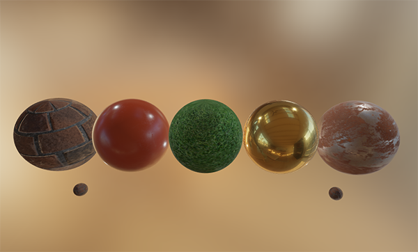
Below you'll see a list of textures you'll frequently find in a PBR pipeline together with its visual output if supplied to a PBR renderer:
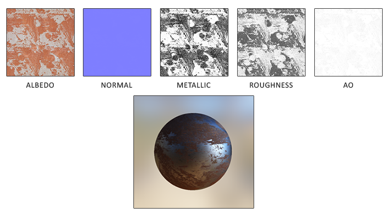
Albedo: the
Normal: the normal map texture is exactly as we've been using before in the normal mapping chapter. The normal map allows us to specify, per fragment, a unique normal to give the illusion that a surface is bumpier than its flat counterpart.
Metallic: the metallic map specifies per texel whether a texel is either metallic or it isn't. Based on how the PBR engine is set up, artists can author metalness as either grayscale values or as binary black or white.
Roughness: the roughness map specifies how rough a surface is on a per texel basis. The sampled roughness value of the roughness influences the statistical microfacet orientations of the surface. A rougher surface gets wider and blurrier reflections, while a smooth surface gets focused and clear reflections. Some PBR engines expect a 1.0 - smoothness) to roughness the moment they're sampled.
AO: the
Artists set and tweak these physically based input values on a per-texel basis and can base their texture values on the physical surface properties of real-world materials. This is one of the biggest advantages of a PBR render pipeline as these physical properties of a surface remain the same, regardless of environment or lighting setup, making life easier for artists to get physically plausible results. Surfaces authored in a PBR pipeline can easily be shared among different PBR render engines, will look correct regardless of the environment they're in, and as a result look much more natural.
Further reading
- Background: Physics and Math of Shading by Naty Hoffmann: there is too much theory to fully discuss in a single article so the theory here barely scratches the surface; if you want to know more about the physics of light and how it relates to the theory of PBR this is the resource you want to read.
- Real shading in Unreal Engine 4: discusses the PBR model adopted by Epic Games in their 4th Unreal Engine installment. The PBR system we'll focus on in these chapters is based on this model of PBR.
- [SH17C] Physically Based Shading, by knarkowicz: great showcase of all individual PBR elements in an interactive ShaderToy demo.
- Marmoset: PBR Theory: an introduction to PBR mostly meant for artists, but nevertheless a good read.
- Coding Labs: Physically based rendering: an introduction to the render equation and how it relates to PBR.
- Coding Labs: Physically Based Rendering - Cook–Torrance: an introduction to the Cook-Torrance BRDF.
- Wolfire Games - Physically based rendering: an introduction to PBR by Lukas Orsvärn.
- [SH17C] Physically Based Shading: a great interactive shadertoy example (warning: may take a while to load) by Krzysztof Narkowi showcasing light-material interaction in a PBR fashion.